Chapter 14 Trend and seasonal fluctuations
Economic and social time series often exhibit systematic patterns beyond random variation. Two of the most important are long-term trends and seasonal fluctuations. Identifying and separating these components helps with interpretation, comparison, and forecasting.
14.1 Components of a time series
A classical time series \(y_t\) can be decomposed into several components:
- Trend (\(T_t\)) – long-term direction of change
- Seasonal component (\(S_t\)) – regular, calendar-related fluctuations
- Irregular component (\(I_t\)) – random and unsystematic variation
Example
We use monthly death data from Statistics Netherlands. In Figure 14.1, we observe evidence of both a trend and annual seasonality, with mortality levels typically higher in winter than in summer.
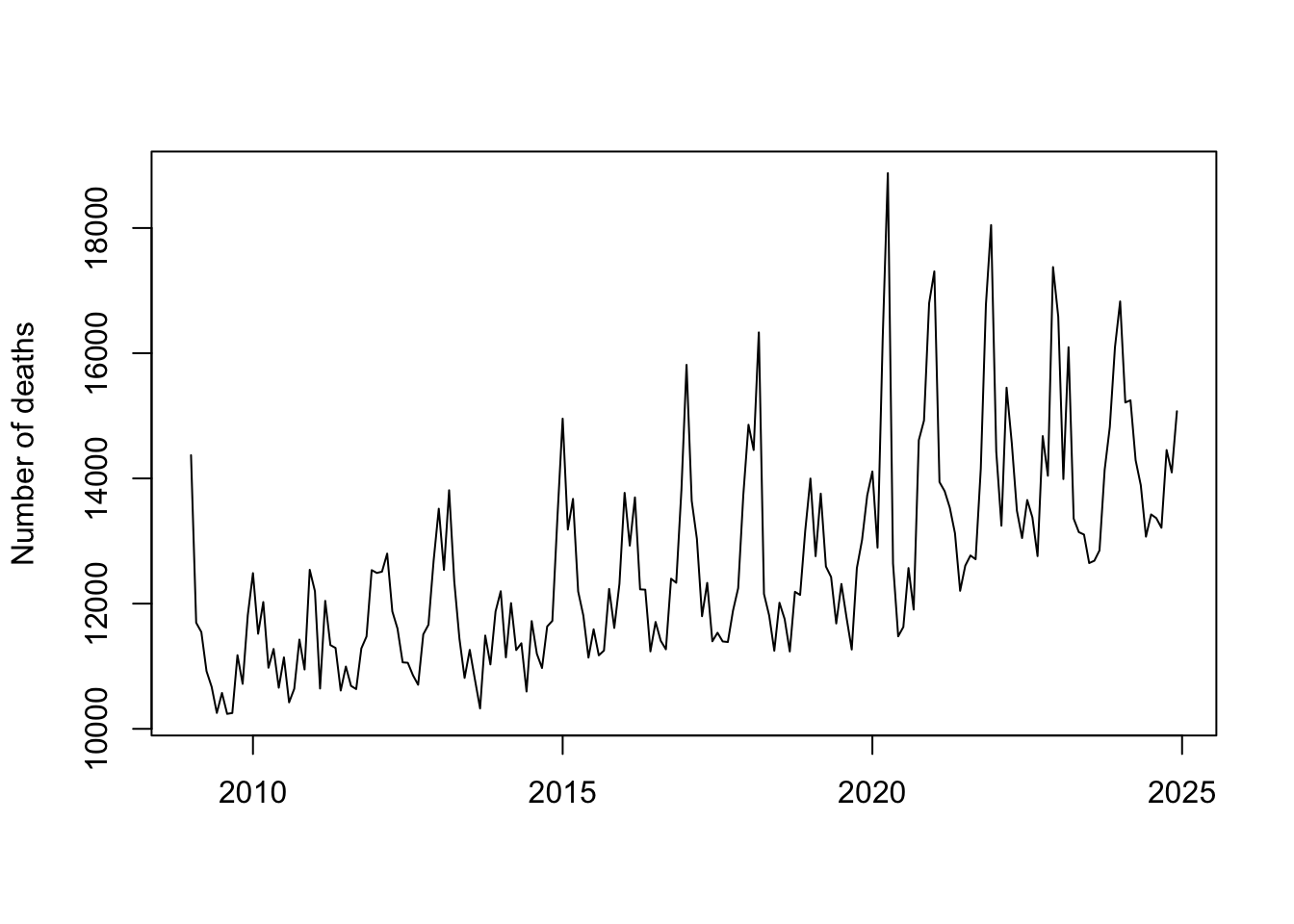
Figure 14.1: Monthly deaths in Netherlands 2009–2024. Source: Statistics Netherlands (https://opendata.cbs.nl/#/CBS/en/dataset/83474ENG/table?dl=24F05)
We use the stl() function from the stats package in R to attempt to decompose the series into trend, seasonal, and irregular components. Results are presented in figure 14.2.
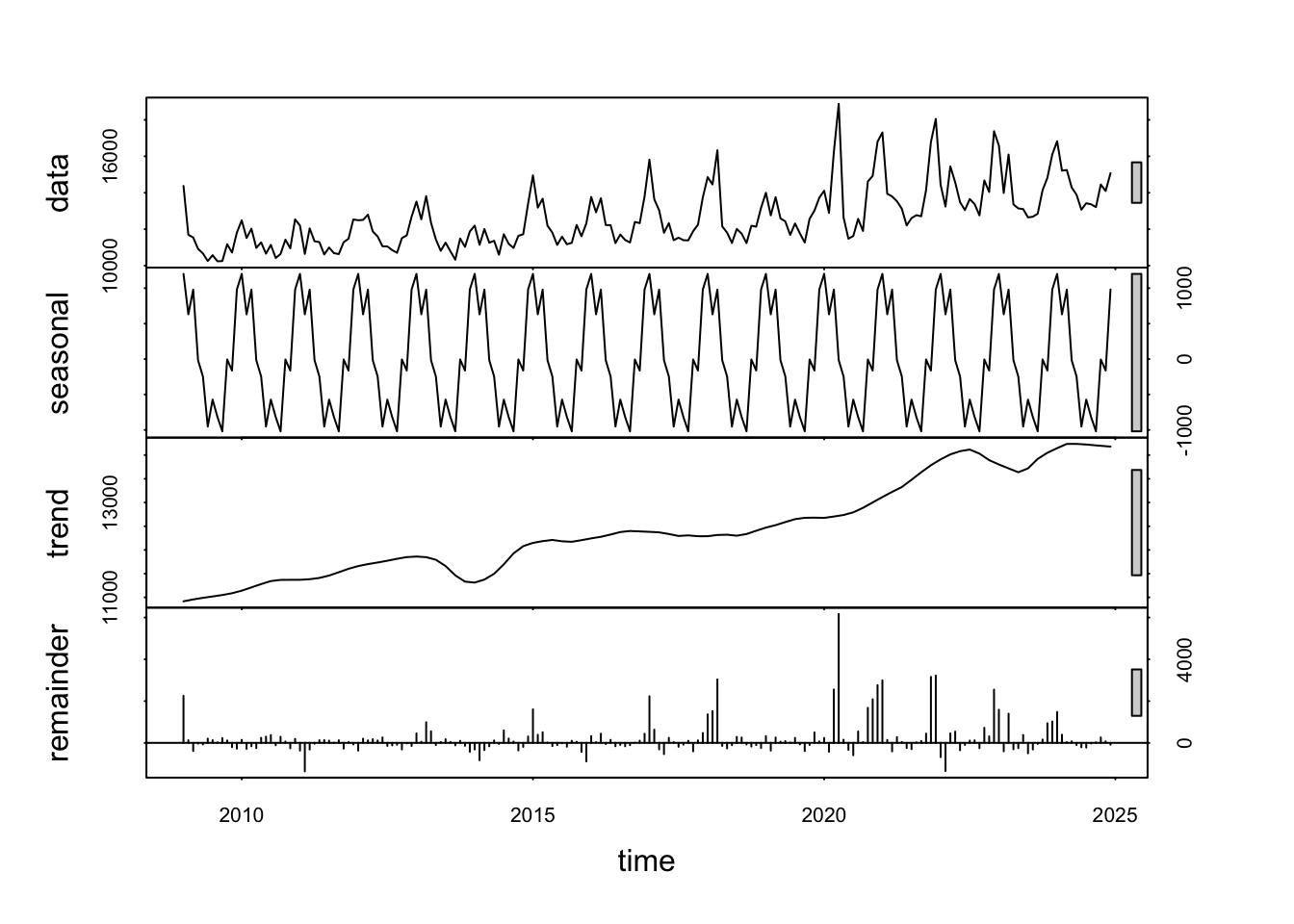
Figure 14.2: Monthly deaths in Netherlands 2009–2024. Decomposition attempt with stl() function in R.
14.3 Linear trend model
A simple parametric representation of trend is the linear trend model:
\[y_t = \alpha + \beta t + \varepsilon_t\]
where:
- \(\alpha\) is the intercept,
- \(\beta\) measures the average change per period.
Interpretation:
- \(\beta > 0\): upward trend
- \(\beta < 0\): downward trend
Linear trends are easy to estimate and interpret, but may oversimplify long time horizons.